Background points
As a last step we prepare the background points (BP) we need to train Maxent. We will use 10,000 background points but not distribute them randomly over the whole study area. Instead we use conditioned latin hypercube sampling
(CLHS) (Minasny & McBratney, 2006) as implemented in the R package clhs. The conditioned latin hypercube sampling distributes the points in a way over the study area that all variables of the environmental data are represented as well as possible.
To do this you first need to download the environmental grids for Ontario, Canada from here if you have not already done it and save them in the layers
folder of your project. You can find the raster files on the OSF page under data/Environment/CAN. Download the complete CAN folder into your data/layers folder and don´t forget to transorm the format to one that is supported by Maxent (see here how to do this). Then execute the script below.
# create 10000 background points for each raster ans use conditioned latin hypercube sampling to distribute points in the best possible way into space | |
# 1 - set up a working-environment #### | |
#------------------------------------# | |
setwd("") # set a working directory | |
# load packages needed | |
require(sf) | |
require(raster) | |
require(clhs) | |
require(dplyr) | |
# 2 - create background points using clhs #### | |
#--------------------------------------------# | |
#load raster | |
r = raster::stack(list.files("data/layers/", full.names=T, pattern=".asc")) | |
raster::crs(r) <- "+proj=longlat +ellps=clrk66 +no_defs +type=crs" | |
# do latin hypercube sampling for 10000 points | |
bg=clhs::clhs(r, size=10000, use.coords = T, simple=F) | |
#save background points as geopackage | |
bg=bg$sampled_data | |
bg=sf::st_as_sf(bg) | |
sf::write_sf(bg, file.path("data/background", "CAN_bg.gpkg")) | |
# get coordinates | |
coords=as.data.frame(sf::st_coordinates(bg)) | |
#transform to one dataframe | |
bg=cbind(data.frame(species="background", lon=coords$X, lat=coords$Y, spatialBlock=1),bg)%>%as.data.frame() | |
#remove geometry information | |
bg$geom<-NULL | |
bg$geometry<-NULL | |
# save as .csv file | |
write.csv(bg,file.path("data/background", "CAN_bg.csv"),row.names = F) | |
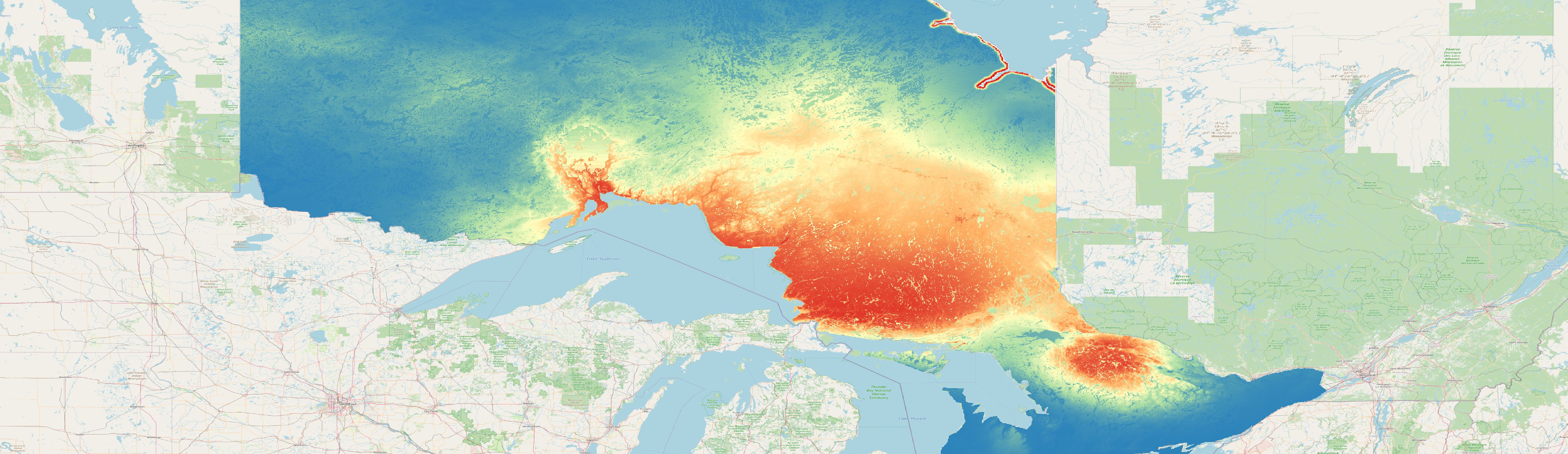
The map shows the distribution of the background points created with conditioned latin hypercube sampling on all environmental layers: