Customizable standalone workflow
To get a quick start with spatialMaxent you can check out the example workflow below. This is especially suitable if you want to understand the functionalities of spatialMaxent and then continue to work on your own data. All data used is obtained from the R package geodata, so you don’t need to download any data beforehand. We will use the bioclimatic variables of the worldclim variables as raster data and model the brown-throated sloth (bradypus variegatus) with south America as study area. Feel free to adapt this for any other region of the world and a species of your choice.
The workflow contains five steps to get the data:
1. Set up your working environment
As a first step set your working directory into a clean folder and create the folder structure as shown in the script below under step one. If you want to change the folder structure, make sure that you also change the paths in the scripts. Also make sure that you have installed the required packages.
2. Download borders of all south american countries
With the function country_codes you can download the codes of the country names of all countries in the world. We filter this dataset to the countries that are in south america and download the polygons of the borders with the function gadm. This vector file is saved with the function writeVector from the terra R package. We need the borders to crop the raster data to our study area.
3. Download bioclimatic variables
We use the bioclimatic variables of the worldclim dataset as environmental variables. They can be downloaded for the whole world with the function worldclim_global. We then clip them to south america and save them as grid files. Make sure that the no data value is set to -9999.
4. Download Bradypus variegatus presence-only data
As presence-only records we download the occurrence data for the species bradypus variegatus. To do this, we use the sp_occurrence function to download data from the Global Biodiversity Information Facility (GBIF). We filter the data to make sure that they are not older than 2000 and that there is not more than one presence only point on a pixel of our grid. Next, we convert the date into an sf object using the function st_as_sf from the R package sf.
5. Part occurrence records in spatial blocks
Finally, we use the R package blockCV to divide the presence points into spatial folds. We create a total of seven spatial folds, five of which are used for training and two for testing. We save the training and test datasets as csv files.
You can see how the spatial folds can look like on the map below:
Full screen version of the map
6. Train spatialMaxent
Now we can create a model with spatialMaxent. For this you can train either with the GUI or from the command line. We need to specify three parameters: First a samples file. In the GUI click the browse button in the upper left corner under Samples and specify the file to train the model (bradypus_variegatus_training.csv). In the command line the file must be specified as samplesfile. We specify the raster files in the GUI on the top right by selecting the directory in which our raster layers are located under the heading Environmental layers, i.e. the layers folder. In the command line we have to specify the path to this folder as environmentallayers. At last we have to specify the location where we want to save the results. To do this, specify the Output directory in the GUI in the lower right area (outputdirectory in the command line).
You can also set the number of threads higher to calculate the forward-variable-selection in parallel.
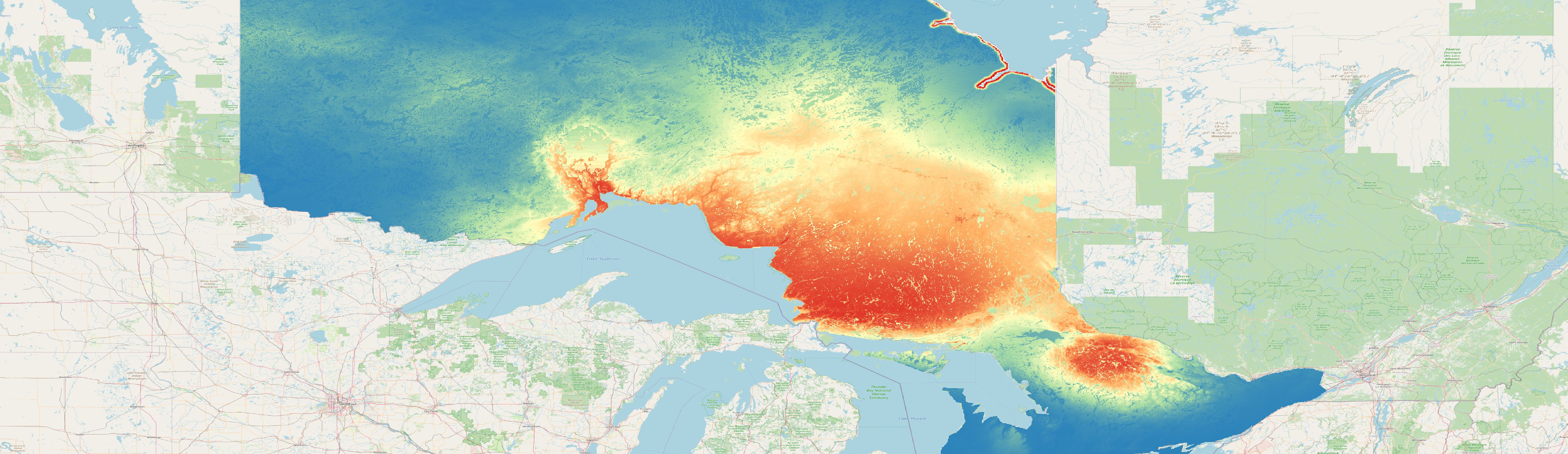
Once your model is finished you can have a look at the prediction raster (map below) and also calculate metrics on the independent test data e.g. Boyce-Index or MAE.