Presence-only data
The species records needed for this exercises can be downloaded via the disdat r-package or over osf.
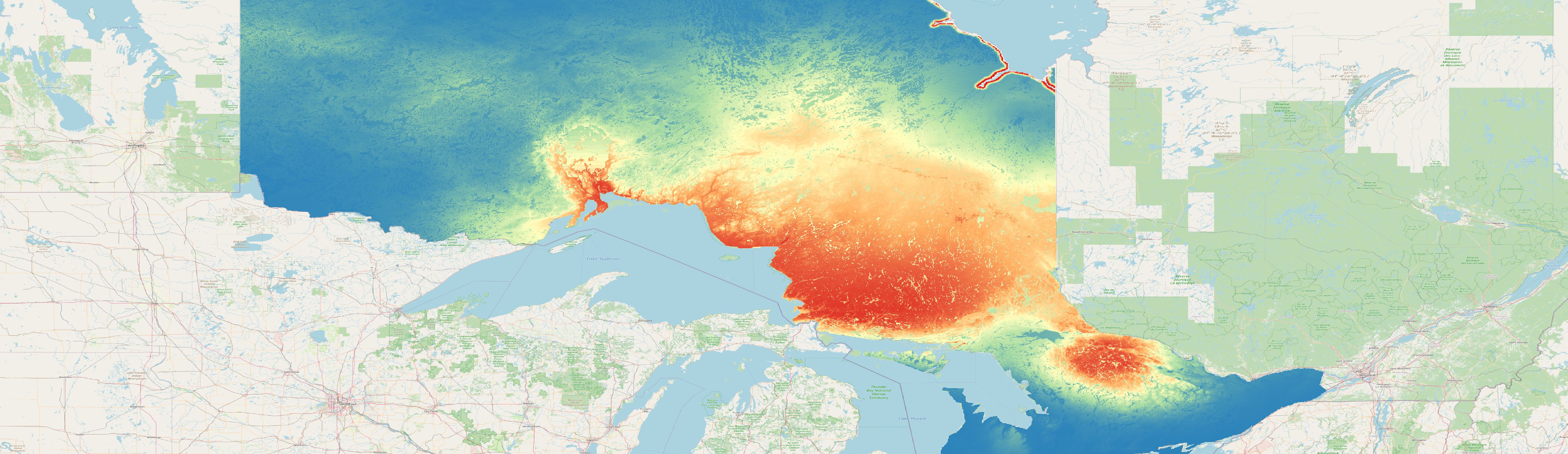
We will not use the presence-absence (PA) and presence-only (PO) data to train and test the models as they are not spatial separated from each other. The presence points of both datasets show a similar pattern that a random partition of train and test data would provide (see map below). Therefore, we will combine the presence points from both datasets into one and part the test and train data ourselves.
Full screen version of the map
Get presence records from PO and PA data
First of all, we will prepare the presence records for this region. Here we use the R package disdat to get the species records. The function disdat::disPo() can be used to derive all PO species records for one region. From this dataframe we can get a total of 20 individual species. As we are not using the (PA) data to evaluate the models we will also use the presence records from the PA data for modeling. To download the PA data we need two different function: the presence and absence information can be downloaded for all species with the function disdat::disPa() the environmental information has to be downloaded separately with the function disdat::disEnv. Note that we will keep only the presence records and will delete the absence records from the dataset.
The script below downloads the data and saves all presence only records for each species individually as geopackage.
For the species can01 you can see the two combined datasets in the map below. In the next exercise we will then part them into spatial folds.